Where We Are
You have collected a great deal, and this chapter is where it pays.
- Chapter 005 turned a house into a vector.
- Chapter 006 asked how many directions a set of arrows really contains, and gave you span, independence and basis.
- Chapter 007 proved that a dot product measures alignment: u⋅v=∥u∥∥v∥cosθ.
- Chapters 008 to 011 gave matrices their algebra — shapes, multiplication, composition, and what one does to space.
Four separate-looking things. They are about to turn out to be one thing.
Today: why the columns of a matrix are the only part you need to understand, what a transformation destroys on the way through, and — at the end — what a single neuron actually computes.
The sentence this chapter exists to earn: a deep neural network is a sequence of learned coordinate systems.
By the end you will not think of a matrix as a grid of numbers again.
The Picture to Hold in Your Head
Now linear algebra becomes neural networks.
A weight vector is a direction the model has learned to care about. The dot product says how strongly an input points along that direction. The bias moves the decision boundary. An activation such as ReLU then folds or clips the space so that the next layer can do something genuinely new.
A layer stacks many learned directions. You can think of its output as a new set of coordinates — not coordinates chosen by humans like “rooms” and “area,” but coordinates learned because they help solve the task.
This also exposes the reason nonlinear activations are essential. Stack linear maps with nothing between them and the product is still one linear map. Depth becomes mathematically fake until something bends the space.
🎛️ Move from What vanishes to One neuron to Two layers, no fold. That sequence is the shortest path from rank and null space to the necessity of nonlinear neural networks.
1. The Discovery: A Matrix Records Where the Basis Lands
Everything so far has been about describing a space. Now we move it.
A linear transformation takes every arrow in the space and sends it somewhere else — stretching, rotating, shearing, or flattening the whole thing at once. We write it x→Ax.
Take
A=[2113],x=[23]
Multiply it out the mechanical way:
Ax=[2(2)+1(3)1(2)+3(3)]=[711]
Fine. The arrow at (2,3) has moved to (7,11). But why there? Arithmetic that you cannot picture is arithmetic you will forget.
So use Chapter 006 §7. Every vector is built from the basis:
x=2e1+3e2
A linear transformation, by definition, respects adding and stretching. So it must be true that
Ax=A(2e1+3e2)=2(Ae1)+3(Ae2)
Now look at what A does to the basis arrows themselves:
Ae1=[2113][10]=[21]Ae2=[2113][01]=[13]
Those are the columns of A. Not a coincidence, not a trick of this example — multiplying by e1 picks out the first column, always.
So:
Ax=2[21]+3[13]=[4+32+9]=[711]✓
Same answer, arrived at with understanding instead of bookkeeping.
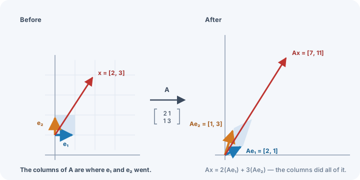
The columns of a matrix tell you where the basis vectors go.
And that is the sentence this chapter was built to deliver. Know where the basis lands, and you know where every single vector in the space lands — because every vector is just some amount of each basis arrow, and the transformation carries those amounts along untouched.
A matrix is not fundamentally a table of numbers. It is a machine that moves a space, and the table is simply the record of where the corner posts ended up.
🎥 Watch this one too. Linear transformations and matrices — 3Blue1Brown, Chapter 3 (11 min). It animates exactly the picture above: a grid deforming while the basis arrows drag it. If one video in this level is worth stopping for, it is this one, and you are now at the precise moment it was made for.
1.1 From Basis Arrows to a Neural Layer: 3 Raw Features → 2 Learned Features
The picture above is not merely a geometric trick. It is almost exactly what a neural-network layer does.
Start with a house described by three normalized measurements:
$
\mathbf{x}
\begin{bmatrix}
\text{size}\
\text{bedrooms}\
\text{age}
\end{bmatrix}
\begin{bmatrix}
0.8\
0.6\
0.2
\end{bmatrix}
$
This is one point in a three-dimensional feature space:
x∈R3.
Its standard basis vectors are
e1=100,e2=010,e3=001.
So the house is really the recipe
$
\mathbf{x}
0.8\mathbf{e}_1
+
0.6\mathbf{e}_2
+
0.2\mathbf{e}_3.
$
Read that slowly:
- 0.8 copies of the size direction,
- 0.6 copies of the bedroom direction,
- 0.2 copies of the age direction.
Now suppose a learned layer wants to replace those three raw measurements with two learned measurements. For intuition, imagine that they eventually behave somewhat like:
- spaciousness-like feature
- modernness-like feature
Those names are only a mental aid. During real training nobody tells the neurons to learn those concepts.
Use the matrix
W=[0.70.20.50.1−0.1−0.8].
Its shape is
W∈R2×3.
So the shape itself tells the story:
R3WR2
Three input coordinates go in. Two output coordinates come out.
Now use the idea from §1: look at the columns first.
W=[0.70.20.50.1−0.1−0.8].
The first column is where e1 goes:
$
W\mathbf{e}_1
\begin{bmatrix}
0.7\
0.2
\end{bmatrix}.
$
The second column is where e2 goes:
$
W\mathbf{e}_2
\begin{bmatrix}
0.5\
0.1
\end{bmatrix}.
$
The third column is where e3 goes:
$
W\mathbf{e}_3
\begin{bmatrix}
-0.1\
-0.8
\end{bmatrix}.
$
So the matrix is saying:
A pure unit of size contributes [0.7,0.2] in the new feature space.
A pure unit of bedrooms contributes [0.5,0.1].
A pure unit of age contributes [−0.1,−0.8].
And because our house was
$
\mathbf{x}
0.8\mathbf{e}_1+0.6\mathbf{e}_2+0.2\mathbf{e}_3,
$
linearity forces
$
W\mathbf{x}
0.8(W\mathbf{e}_1)
+
0.6(W\mathbf{e}_2)
+
0.2(W\mathbf{e}_3).
$
Substitute the three columns:
$
W\mathbf{x}
0.8
\begin{bmatrix}
0.7\
0.2
\end{bmatrix}
+
0.6
\begin{bmatrix}
0.5\
0.1
\end{bmatrix}
+
0.2
\begin{bmatrix}
-0.1\
-0.8
\end{bmatrix}.
$
Now calculate:
$
\begin{bmatrix}
0.56\
0.16
\end{bmatrix}
+
\begin{bmatrix}
0.30\
0.06
\end{bmatrix}
+
\begin{bmatrix}
-0.02\
-0.16
\end{bmatrix}
\boxed{
\begin{bmatrix}
0.84\
0.06
\end{bmatrix}
}.
$
The raw representation
sizebedroomsage
has become a new representation
[0.840.06].
For intuition only, you might read that as
[spaciousness-like scoremodernness-like score].
This is representation learning in miniature: the model is changing the coordinate system in which it describes the same example.
The same matrix has two equally useful readings
Here is the part worth keeping in your head.
Column view — transformation view
column j=Wej
Each column tells you where one input basis direction lands.
For this example:
- column 1 = what a unit of size contributes,
- column 2 = what a unit of bedrooms contributes,
- column 3 = what a unit of age contributes.
Row view — neuron view
The same matrix can be read by rows:
$
W=
\begin{bmatrix}
\text{--- } \mathbf{w}_1^{\mathsf T}\text{ ---}\
\text{--- } \mathbf{w}_2^{\mathsf T}\text{ ---}
\end{bmatrix}
\begin{bmatrix}
0.7 & 0.5 & -0.1\
0.2 & 0.1 & -0.8
\end{bmatrix}.
$
Neuron 1 has weights
w1=0.70.5−0.1
and computes
$
z_1
0.7(0.8)+0.5(0.6)-0.1(0.2)
0.84.
$
Neuron 2 has weights
w2=0.20.1−0.8
and computes
$
z_2
0.2(0.8)+0.1(0.6)-0.8(0.2)
0.06.
$
So:
$
W\mathbf{x}
\begin{bmatrix}
\mathbf{w}_1^{\mathsf T}\mathbf{x}\
\mathbf{w}_2^{\mathsf T}\mathbf{x}
\end{bmatrix}
\begin{bmatrix}
0.84\
0.06
\end{bmatrix}.
$
That gives one matrix two complementary meanings:
Columns:Rows:where the old basis directions gowhat direction each neuron measures
These are not two different operations. They are two views of the same transformation.
Mental model: the columns explain how the old coordinates are rebuilt in the new space; the rows explain what each new neuron measures from the old space.
Why two neurons?
Because each neuron produces one scalar:
z1=w1Tx,z2=w2Tx.
Two neurons therefore produce two output coordinates:
3 input features→2 neurons→2 output features
If the layer had three neurons, its weight matrix would have three rows,
W∈R3×3,
and it would produce three output numbers. To deliberately go from three features to two, you need two output neurons in this column-vector convention.
Convention note. Some code and textbooks store a batch of examples as rows and write xW instead of Wx. Then the weight matrix is transposed and neurons appear as columns. Nothing mathematical changed — only the storage convention did. In this chapter we keep column vectors so that “column j = where ej goes” stays visually exact.
2. Rank: How Many Directions Survive the Trip
A transformation does not have to be kind. It can flatten.
Ask Chapter 006’s span question about the columns of a matrix, because the columns are where everything ends up: what do the columns span? That answer has a name.
Rank = the number of independent directions among the columns = the dimension of what comes out.
For A in §1, the columns [2,1] and [1,3] point differently, so they span the plane. Rank 2. Nothing was lost.
Now this one:
B=[1224]
The columns are [1,2] and [2,4] — and the second is exactly twice the first. One direction wearing two hats, which is Chapter 006 §5 all over again. Rank 1.
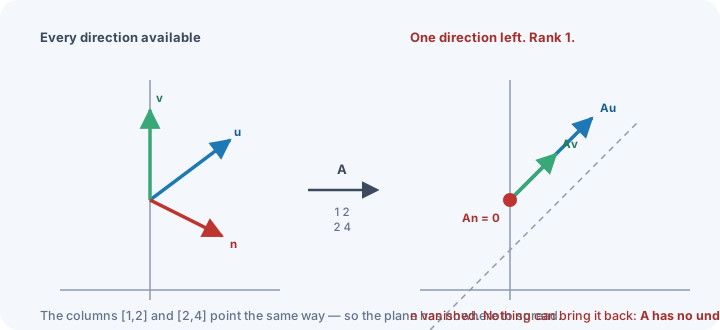
Feed the whole plane through B and every output lands on a single line. A two-dimensional space went in; a one-dimensional space came out. The transformation had nowhere to put the rest.
A matrix with the most rank it could possibly have is called full rank. Less than full rank means the output space is smaller than the input space — and something was thrown away on the journey.
If a 2-D plane arrives as a 1-D line, a whole direction’s worth of input had to disappear. Which one?
Solve Bn=0 for the B above:
[1224][n1n2]=[00]⟹n1+2n2=0
So anything along n=[2,−1] is sent to the origin and obliterated. Check: 1(2)+2(−1)=0 ✓ and 2(2)+4(−1)=0 ✓.
That set — everything crushed to zero — is the null space.
And now the consequence that matters. Suppose someone hands you an output and asks what went in. Both x and x+n produce it, because the n part contributed nothing:
B(x+n)=Bx+Bn=Bx+0=Bx
There is no way to tell which one it was. Not “it’s hard” — the information is gone.
A transformation can be undone only if it destroys nothing. Null space bigger than a point means no inverse exists, ever.
The bookkeeping is exact, and it is called rank–nullity:
directions that survivedrank+directions crushednullity=directions you started withd
For B: rank 1 + nullity 1 = 2. ✓ Every direction is accounted for. Nothing leaks.
This is the exact arithmetic behind a bottleneck layer in a neural network — a layer that maps 512 numbers down to 32. Rank at most 32, so at least 480 directions of input are being deliberately thrown away. Sometimes that is the point (compression). Sometimes it is a bug you cannot see.
4. Near Dependence: The Trouble That Does Not Announce Itself
Exact dependence is the easy case. The dangerous case is almost.
Return to Ramesh’s sheet from Chapter 006 one more time, and look closely at what is actually written in it. Square metres were recorded to one decimal place: 74.3, 111.5, 83.6, 148.6. But 800×0.0929=74.32, not 74.3. Somebody rounded.
So the two columns are not exactly proportional. Not quite dependent. Which means:
- The rank is technically full. No error. No warning. Nothing to catch.
- But the second direction is so nearly a copy of the first that it carries almost nothing.
- And the dials for those two columns can swing wildly in opposite directions and barely change the prediction — which is precisely the instability that opened Chapter 006, where two training runs disagreed and scored the same.
This is the condition number from Chapter 005 §10, arriving from the other side. There, mismatched units stretched the loss valley into a canyon. Here, near-duplicate columns do the same thing — a direction so flat that the model can slide along it for free.
Exact dependence fails loudly and is easy to fix. Near dependence fails quietly and is not. When a model’s weights change dramatically between runs while the loss does not, this is the first thing to suspect.
5. 🎯 The Discovery: A Neuron Is One Learned Direction
Everything is now in place. Here is what it was for.
A neuron, stripped of decoration, computes
z=w1x1+w2x2+⋯+wdxd+b=w⋅x+b
Set the bias aside for a moment and look at the shape of it. With x∈R2 and one output:
R2⟶R1
A whole two-dimensional space arriving as one number. By §2 that is a rank-1 transformation, and by §3 almost everything about the input is being thrown away. The neuron keeps exactly one thing.
Which thing? Chapter 007 proved it and we can finally spend it:
w⋅x=∥w∥∥x∥cosθ
Strip out the sizes — Chapter 006 §11’s move — and what is left is direction. So the neuron is asking one question, and the same question every time:
“How strongly does this input point in my direction?”
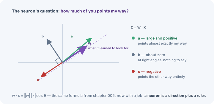
| What comes out | What it means |
|---|
| large positive | the input points almost exactly along w |
| near zero | at right angles — this input has nothing to do with what the neuron looks for |
| negative | the input points the other way |
And w is learned. Nobody writes it down. Gradient descent moves it until it points somewhere useful.
Suppose a neuron settles on w=[0.8,0.6]. In a house model that direction might come to mean “large and modern”. Deep in an image network, the learned directions in the first layer reliably come to mean things like vertical edge or patch of curve; later layers point along eye-like texture or wheel.
Neuron=a learned direction+a ruler for measuring along it
Look back at Chapter 006 §14: in an orthonormal basis, a coordinate is a dot product with a direction. A neuron computes a dot product with a direction. A neuron is computing a coordinate — in a basis the machine is choosing for itself.
6. A Layer Is a New Basis the Machine Chose
One coordinate is not a description. You need several.
So use several neurons. Take an input with three measurements and four neurons, each with its own learned direction:
z1=w1⋅x,z2=w2⋅x,z3=w3⋅x,z4=w4⋅x
Four separate lines, each doing the same kind of work. Chapter 005 met this problem already — many things of the same shape, wanting one name. Stack the weight vectors as rows:
W=————w1Tw2Tw3Tw4T————⟹z=Wx+b
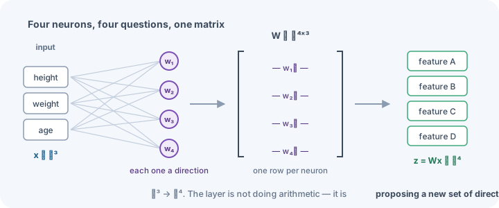
The shapes say it exactly: x∈R3, W∈R4×3, z∈R4. The layer performs
R3⟶R4
Now read that with Chapter 006 §12 and §1 in hand, and it stops being arithmetic:
A layer is not computing numbers. It is proposing a new set of directions to describe the input in — and then reporting the input’s coordinates in them.
Your house arrived described as height, weight, age — coordinates in a basis that a clerk chose because those were easy to write down. It leaves described as four numbers in a basis the machine chose, because that basis makes the next step easier.
7. 🔬 The Experiment: Why Stacking Layers Alone Does Nothing
Predict before you read on. A layer is z=Wx. Stack a hundred of them, one after another. You now have a hundred matrices and a great many dials. Is the resulting machine more powerful than one layer? Commit to an answer.
Push a vector through three layers:
h1=W1x,h2=W2h1,h3=W3h2
Substitute:
h3=W3(W2(W1x))=(W3W2W1)x
Matrix multiplication is associative, so those three multiply together into one matrix:
W=W3W2W1⟹h3=Wx
A hundred layers collapse the same way. A hundred stacked linear layers are exactly one linear layer — you can find the single matrix that does the identical job, and it is no bigger than the ones you started with.
Run it in the notebook. Multiply a hundred random matrices together, compare against passing a vector through them one at a time, and watch the answers agree to machine precision. Every parameter after the first layer bought nothing.
Now the geometric version of why that is fatal:
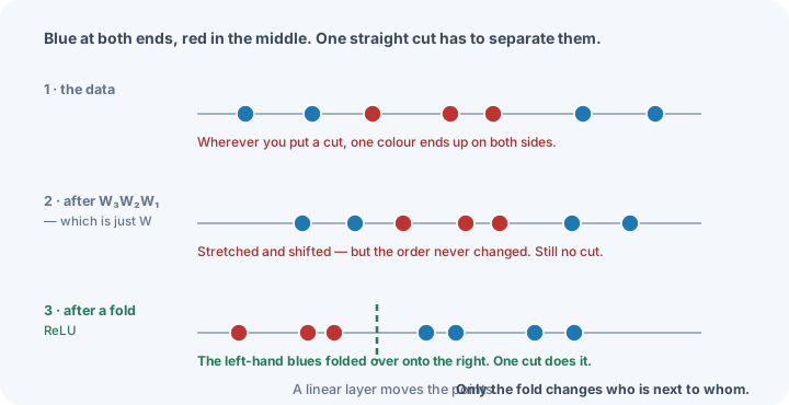
A linear transformation can stretch, rotate, shear and flatten. What it cannot do is change who is next to whom. Points that started in a tangled order stay in a tangled order, however violently you stretch them.
So add something that is not linear. The usual choice is ReLU:
ReLU(z)=max(0,z)
which simply flattens everything negative to zero — and that is a fold. Two different inputs can now land in the same place, which no amount of stretching could ever arrange. A real layer is therefore
h=σ(Wx+b)
| Piece | What it does |
|---|
| Wx | move the space — the learned directions of §6 |
| +b | shift it |
| σ | fold it — the only step that can reorder |
Stack those and the layers stop collapsing, because there is a fold between each pair that no single matrix can imitate.
This is why activation functions exist. Not as a detail of the recipe — as the entire reason depth buys you anything at all.
8. 🎯 Machine Learning Connection: Learning Better Coordinates
Put the whole chain in one place:
| Idea | What it turned out to be |
|---|
| Span | what a set of directions can reach |
| Independence | whether any of them is wasted |
| Basis | exactly enough directions, no more |
| Coordinates | how much of each — instructions, not the thing |
| Matrix | the record of where the basis landed |
| Rank | how many directions survived |
| Dot product | how much of this lies along that |
| Neuron | one learned direction, plus a ruler |
| Layer | a whole new basis, chosen by the machine |
| Activation | the fold that makes depth mean something |
And the sentence it all adds up to:
A deep neural network is a sequence of learned coordinate systems.
Each layer asks the same question: can I re-describe this so that the next step becomes easy? Nothing more mystical than that.
For an image, the re-describing runs roughly:
pixels→edges→textures→shapes→parts→“cat”
For language:
tokens→embeddings→context→meaning→the next word
At every arrow the data is being handed a better basis than the one it arrived in. That is the work.
So this level is not mathematics you must get through before the interesting part. You have been reading the interesting part. Span, basis, rank and the dot product are not preparation for neural networks — they are what neural networks are made of.
9. How It Breaks
| Failure | What it looks like | Why |
|---|
| An accidental bottleneck | a layer silently destroying signal | §3. Rank lower than you assumed, and the null space is carrying real information away. |
| Near dependence in the inputs | weights swing between runs, loss unmoved | §4. Full rank on paper, a flat direction in practice. |
| No activation | a deep model no better than a shallow one | §7. W3W2W1=W. Every layer after the first bought nothing. |
| A dead neuron | one output stuck at zero for every input | ReLU with weights pointing where no data goes. Its direction measures nothing, and the gradient cannot revive it. |
| Reading a matrix as a table | no intuition for what a layer did | §1. The grid is the receipt. The transformation is the thing. |
10. Distinctions That Matter
| A matrix — the record | A transformation — what it does to space |
| Column space — where outputs can land | Null space — what is destroyed getting there |
| Rank — directions that survive | Nullity — directions crushed |
| Linear — can stretch, cannot reorder | Non-linear — can fold, so can reorder |
| A neuron — one learned direction | A layer — a whole basis of them |
| Given coordinates — the clerk’s choice | Learned coordinates — the machine’s choice |
11. What We Discovered
- A matrix is not fundamentally a table. Its columns record where the basis vectors land, and that fixes where every other vector lands.
- Because Ax=x1(Ae1)+⋯, understanding a transformation means understanding d arrows, not d2 numbers.
- Rank counts the directions that survive the trip; the null space is what the trip destroys.
- Rank plus nullity always equals what you started with. Nothing leaks.
- A transformation that destroys anything cannot be undone — not “is hard to undo”, cannot.
- Near-dependence is full rank and still ruinous, and it never announces itself.
- A neuron is one learned direction plus a ruler: how much of this input lies along the thing I learned to look for?
- A layer stacks those directions into W and returns the input’s coordinates in a basis the machine chose.
- Stacked linear layers collapse into a single matrix. The activation is a fold, and folding is the only operation that can change which points sit next to which.
- Therefore: a deep network is a sequence of learned coordinate systems, each one chosen to make the next step easier.
12. Mathematics We Built
Ax=x1(Ae1)+x2(Ae2)+⋯+xd(Aed)
rank(A)+nullity(A)=dN(A)={x:Ax=0}
z=w⋅x+bz=Wx+bh=σ(Wx+b)
W3W2W1=W(why depth needs σ)
13. What Each Symbol Means
| Symbol | In English | In code |
|---|
| Aei | where the i-th basis arrow lands — column i | A[:, i] |
| rank(A) | independent directions among the columns | np.linalg.matrix_rank(A) |
| N(A) | the null space — inputs sent to zero | scipy.linalg.null_space(A) |
| W | a layer’s weights, one row per neuron | W |
| b | the bias — one per neuron | b |
| σ | the activation — the fold | np.maximum(0, z) |
| Rm×n | m rows, n columns | shape (m, n) |
| h | the new representation | h |
14. One-Minute Explanation
Explain to someone with no mathematics, using no equations:
What is a neuron actually doing, and why does a network need more than one layer?
15. Exercises
Level 1 — Observe. Look at the two panels in §1. Before the transformation, the shaded region is a square. After, it is a slanted parallelogram. Which two arrows decided its new shape, and where in the matrix are they written down?
Level 2 — Calculate (by hand). For A=[2113]: compute Ae1 and Ae2 and confirm they are the columns. Then compute A[1−1] twice — row by row, and as 1(Ae1)+(−1)(Ae2). Repeat both for B=[1224], find a non-zero n with Bn=0, and state the rank and nullity of each.
Level 3 — Derive. Prove that a linear map from R3 to R2 must have a non-trivial null space, whatever its entries. Then prove that if A has a non-trivial null space, no matrix C can satisfy CA=I. Finally, show that the composition of two linear maps is linear — which is the fact §7 leans on.
Level 4 — Investigate (notebook). Multiply a hundred random 4×4 matrices into a single W, and confirm that pushing a vector through the stack one layer at a time gives the same answer as Wx, to machine precision. Then insert a ReLU between each pair and show it no longer does. Finally, take the tangled one-dimensional data from §7 and find weights for a two-neuron layer with ReLU that makes the two colours linearly separable.
Level 5 — Design. You are designing a layer that maps 512 numbers down to 32. By §3 you are deliberately destroying at least 480 directions of input. Decide what you want that layer to keep and what you are content to lose, and say how you would test — after training — whether it threw away something it needed. Then answer the harder question: if it did, what would that look like in the model’s behaviour, and how would you tell it apart from simply not having trained long enough?
16. Common Mistakes
| Mistake | Why it is wrong |
|---|
| “A matrix is a table of numbers.” | It is a record of where the basis landed. The table is the receipt, not the thing. §1. |
| “Rank is about the size of the matrix.” | A 1000×1000 matrix can have rank 1. Rank counts independent directions, not rows. §2. |
| “If the rank is full, the data is fine.” | Near-dependence is full rank and still ruinous — and silent. §4. |
| “A neuron recognises an object.” | A neuron measures alignment with one direction. Whatever meaning that direction has was learned, and it is one number. §5. |
| “More layers is more power.” | Not without a non-linearity. W3W2W1=W. §7. |
| “The activation is there to squash numbers into a range.” | Some do. The reason they are necessary is that only a fold can reorder points. §7. |
| “Destroying information is a bug.” | A layer that maps 512 to 32 destroys on purpose. Choosing what to lose is most of what representation learning is. §3, §8. |
17. Socratic Questions
- A matrix has 10,000 entries. How many arrows do you actually have to understand to know what it does, and why?
- Is a layer that maps 512 numbers to 32 destroying information or choosing what to keep? Does the distinction change anything you would do?
- A single neuron measures alignment with one direction. What can it never detect, however it is trained?
- Would you want a layer’s learned directions to be orthonormal? What would you gain, and what might you give up?
- ReLU folds, and a fold cannot be undone. So every layer destroys information deliberately. How can destroying information make a model better?
- §7 showed that linear layers collapse. Does that mean a linear model is useless — or are there problems where the collapse costs you nothing?
18. 🔭 Bridge to Chapter 014
We now know that a matrix moves space, and that the columns say how.
But some directions are more interesting than others. Push most arrows through A and they come out pointing somewhere new. A few come out pointing exactly where they started, only longer or shorter.
Those directions are special, and they are special in a way that matters enormously: they are the directions along which a repeated transformation grows or dies. Apply A a hundred times and what survives is decided entirely by them — which is the whole story of why deep networks explode or vanish during training.
Which arrows does a transformation leave pointing the same way?
That is where Chapter 014 begins.
What You Will Need, and When
Linear algebra — the rest of this level
Chapters 014 to 016 find the special directions of a transformation, factorise any matrix into rotate–stretch–rotate, and finally ask the data to hand you its own best basis.
🎥 Watch this now — Linear transformations and matrices, 3Blue1Brown, Chapter 3 of Essence of Linear Algebra (11 min). It animates §1 exactly: a grid deforming while the basis arrows drag it along. If you watch one video in this level, this is the one, and this is the moment.
Differential calculus — when you ask how the directions get learned
All chapter we have said w is learned and moved straight on. How?
The machine nudges every weight a little, in whichever direction lowers the loss — Chapter 001’s compass, now pointed at a matrix instead of a single dial. Doing that for millions of weights at once, across a stack of layers with folds in between, needs the chain rule and the algorithm built on top of it.
→ Level 02, from Chapter 017.
🎥 Neural Networks — 3Blue1Brown. Its third and fourth videos show gradient descent and backpropagation running over exactly the W you built in §6.
References
The matrix-as-transformation framing
3Blue1Brown, Linear transformations and matrices — Chapter 3 of Essence of Linear Algebra.
https://youtu.be/kYB8IZa5AuE
The sentence “the columns of a matrix tell you where the basis vectors land” is Grant Sanderson’s, and it is the single most useful sentence in elementary linear algebra.